As part of Quantum's retail analytics team, I was tasked with helping our client understand the type of customers and their purchasing behavior.

Task - Data preparation and customer analytics

Client - The Category Manager for Chips

Objective - To better understand the types of customers who purchase Chips and their purchasing behavior within the region.

Tools – R

Deliverables

• Define recommendations from the insights,

• Determine which segments should be targeted,

• Determine if packet sizes are relative. Etc.

Data Exploration

Process

The first step in any analysis is to first understand the data and to do that the datasets were imported into R studio but nothing can be done without first installing and loading some important libraries needed for this analysis, so to get that done, the install() and library() functions were used to install and load the following libraries - data.table, ggplot2, ggmosaic, readr, dplyr, stringr.

To understand what these libraries do, an explanation is given below:

data.table - data.table is a powerful package in R that provides enhanced functionality for data manipulation and analysis. It offers fast data processing capabilities and efficient handling of large datasets, making it ideal for working with large-scale data operations.

ggplot2 - ggplot2 is a widely-used data visualization package in R. It provides a flexible and elegant syntax for creating a wide range of static and interactive plots. With ggplot2, you can easily customize plot aesthetics, map variables to different visual properties, and create visually appealing data visualizations.

ggmosaic - ggmosaic is an extension package for ggplot2 that specializes in creating mosaic plots. Mosaic plots are useful for visualizing the relationship between two categorical variables, showing the distribution and proportions of observations within each category.

readr - readr is a package in R that offers efficient and user-friendly functions for reading structured data files, such as CSV, TSV, and fixed-width files. It provides faster and more reliable methods for importing data into R compared to base R functions, with automatic type inference and better handling of various data formats.

dplyr - dplyr is a popular package in R for data manipulation and transformation. It provides a concise and intuitive grammar of data manipulation functions, allowing you to easily filter, arrange, summarize, and mutate data. dplyr enables efficient data wrangling tasks, making it a valuable tool for data preprocessing and analysis.

stringr – stringr is a package in R that offers a set of functions for working with strings. It provides convenient methods for string manipulation, pattern matching, and text extraction. With stringr, you can efficiently clean and preprocess textual data, perform string operations, and handle regular expressions.

The datasets provided by the client were imported into R studio using the following code below:

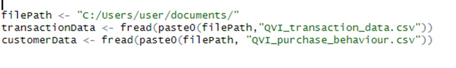
The location of the datasets was saved into a data.table called filepath which was later used to load both datasets and saved them into individual data.tables called transactionData and customerData.

Examining transaction data

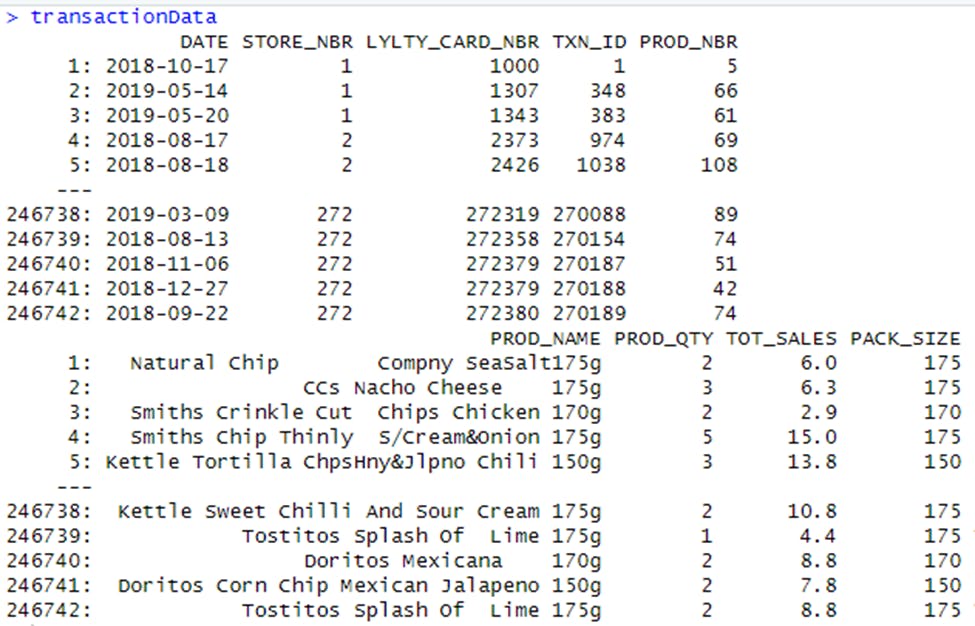
Now that both datasets have been imported, the analysis can begin by taking a look at each of the datasets provided starting with the transaction dataset.

The str() function was used to look at the format of each column and also to see a sample of the data. As the dataset has been read in as a data.table, transactionData was passed into the str() function to see the format of each column and was also passed into the head() function to see a sample of the first 10 rows of the data.

From the image above, the date column is in an integer format instead of a data format. That has to be changed and the following line of code was used:

transactionData$DATE <- as.Date(transactionData$DATE, origin = "1899-12-30")

The result of the above line of code is shown in the image below which clearly shows that the data column is now in the right format.

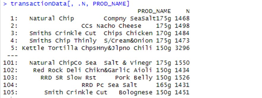
To better understand the data being worked on, the transactionData[, .N, PROD_NAME] code was used to look at the product name. It appears the products are potato chips but to be sure they are all chips, some basic text analysis was done by summarizing the individual words in the product name.

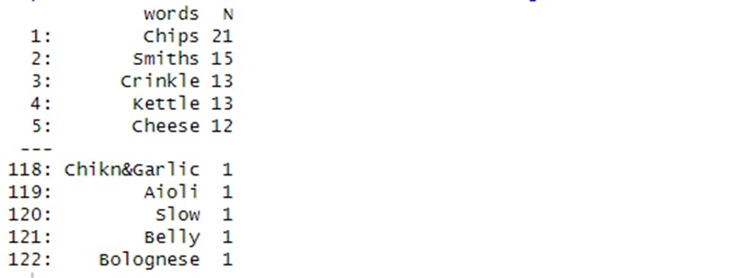
It appears there are some salsa products in the dataset but since the chips category is the only category of interest, these products were removed. Next, the summary() function was used to check summary statistics such as mean, min and max values for each feature to see if there are any obvious outliers in the data and if there are any nulls in any of the columns.

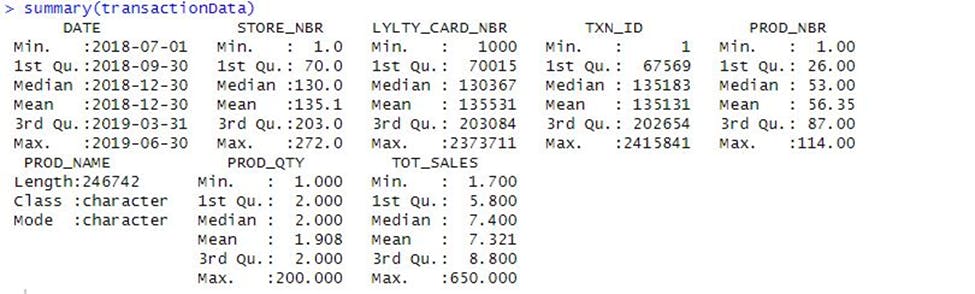
There are no nulls in the columns, but product quantity appears to have an outlier which led to further investigation to see where 200 packets of chips are bought in one transaction. There are two transactions where 200 packets of chips are bought in one transaction and both of these transactions were by the same customer.

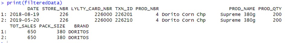
It looks like this customer has only had two transactions over the year and is not an ordinary retail customer. The customer might be buying chips for commercial purposes instead therefore will be removed from further analysis. To confirm the outlier has been removed, the summary of the data was checked again and it looks better now.

The number of transactions over time was looked at next to see if there are any obvious data issues such as missing data.

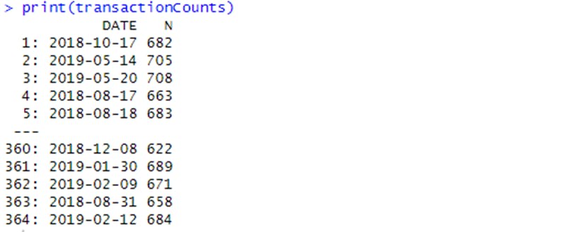
The number of transactions was counted by date and there are only 364 rows, meaning only 364 dates which indicate a missing date. To locate the missing data, a sequence of dates from 1 Jul 2018 to 30 Jun 2019 was created and used to create a chart for the number of transactions over time to find the missing date.

From the chart, there is a sharp increase in purchases in December and a break in late December. Further investigation was done to understand why that break happened by zooming in and focusing on December sales. There's an increase in sales in the lead-up to Christmas and there are zero sales on Christmas Day itself. This is due to shops being closed on Christmas Day and that happens to be the missing date in the dataset.

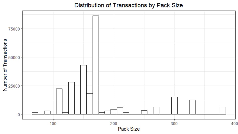
With data no longer having outliers, some other features such as the brand of chips and pack size were created from the PROD_NAME column. The pack size was first derived and from the image below, the largest size is 380g and the smallest size is 70g which seems sensible!

The dataset was checked to confirm if indeed pack sizes have been picked out and the image below sees it has been picked out.

The distribution of transactions by pack size was looked at and the 170g pack size is the most popular size purchased among customers.

Next is to create brands and to accomplish this, the first word in PROD_NAME was used to work out the brand name. Note, this might not seem reasonable but it’s the best way to derive it for the analysis.

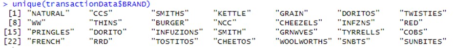
Some of the brand names look like they are of the same brands - such as RED and RRD, which are both Red Rock Deli chips. So, they were combined and the same was done for every other brand as well.

That brings the data exploration of the transaction data to an end and the beginning of the data exploration of the customer data.

Examining customer data

With the transaction dataset cleared and ready for analysis, the customer dataset was checked out for some basic summaries of the dataset, including distributions of any key columns.

With the satisfaction that the customer dataset is okay and perfect, both datasets were merged and from the resulting file, the number of rows in the new dataset called Data is the same as that of transactionData which means no duplicates were created. This is because the Data file was created by setting all.x = TRUE (i.e. a left join) which means taking all the rows in transactionData and finding rows with matching values in shared columns and then joining the details in these rows to the first mentioned table.

To be sure all customers were included, and some weren't skipped, null values were checked for and as shown below, there are no nulls! So, all our customers in the transaction data have been accounted for in the customer dataset.

This concluded the data exploration part of the analysis and the new file was exported because it will be needed later during the analysis.

Now that the data is ready for analysis, some metrics of interest were defined according to the client's needs. Some of these metrics are:

• Who spends the most on chips (total sales), describing customers by lifestage and how premium their general purchasing behavior is?

• How many customers are in each segment?

• How many chips are bought per customer by segment?

• What's the average chip price by customer segment? Etc.

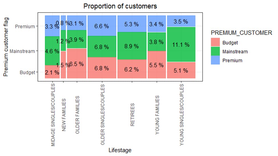
A calculation for the total sales by LIFESTAGE and PREMIUM CUSTOMER was done and the split by these segments was plotted to describe which customer segment contributes most to chip sales.

From the image above, it’s clear that sales are coming mainly from Budget - older families, Mainstream - young singles/couples, and Mainstream - retirees. Further drilling was done to see if the higher sales are due to there being more customers who buy chips and there are more Mainstream - young singles/couples and Mainstream - retirees who buy chips. This contributes to there being more sales to these customer segments, but this is not a major driver for the Budget - Older Families segment as shown below.

Higher sales may also be driven by more units of chips being bought per customer and that was checked out as well. Older families and young families in general buy more chips per customer

The investigation into the average price per unit of chips bought for each customer segment shows that it is also a driver of total sales and MAINSTREAM MIDAGE and YOUNG SINGLES AND COUPLES are more willing to pay more per packet of chips compared to their budget and premium counterparts. This may be due to premium shoppers being more likely to buy healthy snacks and when they buy chips, this is mainly for entertainment purposes rather than their own consumption. This is also supported by there being fewer PREMIUM MIDAGE and YOUNG SINGLES AND COUPLES buying chips compared to their mainstream counterparts.

As the difference in average price per unit isn’t large, a check to see if this difference is statistically different was performed by running an independent t-test.

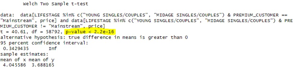
The t-test results in a p-value < 2.2e-16, i.e. the unit price for mainstream, young and mid-age singles and couples are significantly higher than that of budget or premium, young and mid-age singles and couples.

Deep dive into specific customer segments for insights

A recommendation to the client is to target customer segments that contribute the most to sales to retain them or further increase sales. Mainstream - young singles/couples falls into this bracket and a deep dive was done to find out if they tend to buy a particular brand of chips.

The image above shows that:

• Mainstream young singles/couples are 23% more likely to purchase Tyrrells chips compared to the rest of the population

• Mainstream young singles/couples are 56% less likely to purchase Burger Rings compared to the rest of the population.

To find out if the target segment tends to buy larger packs of chips, the pack proportion was done and Mainstream young singles/couples are 27% more likely to purchase a 270g pack of chips compared to the rest of the population.

Lastly, to figure out what brand sells this pack size, a drill down was done and Twisties are the only brand offering 270g packs and so this may instead be reflecting a higher likelihood of purchasing Twisties.

Recommendation

1. Target Mainstream - young singles/couples segment: This segment contributes significantly to chip sales. To retain and further increase sales, the client should focus on this customer segment by offering targeted promotions and marketing campaigns.

2. Promote Tyrrells chips: Among the Mainstream - young singles/couples segment, Tyrrells chips have a higher likelihood of purchase. The client should emphasize and promote Tyrrells chips to this specific segment to capitalize on their preference.

3. Highlight 270g pack size: Mainstream - young singles/couples are more likely to purchase larger pack sizes, particularly the 270g pack. Twisties is the only brand offering this pack size, so the client should ensure the visibility and availability of Twisties in stores targeting this customer segment.

4. Monitor pricing strategy: Mainstream - young and mid-age singles/couples are willing to pay higher prices per packet of chips compared to other segments. The client should consider adjusting pricing strategies to maximize profitability while maintaining competitive prices.

5. Further analysis was conducted to explore additional factors that influence Chips sales.

   Read the article here

   By implementing these recommendations, the client can optimize their chip sales strategy, increase customer satisfaction, and drive overall business growth.